2D examples
These examples require raw data which are automatically
downloaded from the source repository by the script
example_helper.py.
Please make sure that this script is present in the example
script folder.
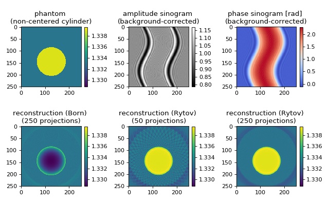
Mie off-center cylinder
The in silico data set was created with the softare miefield. The data are 1D projections of an off-center cylinder of constant refractive index. The Born approximation is error-prone due to a relatively large radius of the cylinder (30 wavelengths) and a refractive index difference of 0.006 between cylinder and surrounding medium. The reconstruction of the refractive index with the Rytov approximation is in good agreement with the input data. When only 50 projections are used for the reconstruction, artifacts appear. These vanish when more projections are used for the reconstruction.
backprop_from_mie_2d_cylinder_offcenter.py
  1import matplotlib.pylab as plt
  2import numpy as np
  3
  4import odtbrain as odt
  5
  6from example_helper import load_data
  7
  8
  9# simulation data
 10sino, angles, cfg = load_data("mie_2d_noncentered_cylinder_A250_R2.zip",
 11                              f_sino_imag="sino_imag.txt",
 12                              f_sino_real="sino_real.txt",
 13                              f_angles="mie_angles.txt",
 14                              f_info="mie_info.txt")
 15A, size = sino.shape
 16
 17# background sinogram computed with Mie theory
 18# miefield.GetSinogramCylinderRotation(radius, nmed, nmed, lD, lC, size, A,res)
 19u0 = load_data("mie_2d_noncentered_cylinder_A250_R2.zip",
 20               f_sino_imag="u0_imag.txt",
 21               f_sino_real="u0_real.txt")
 22# create 2d array
 23u0 = np.tile(u0, size).reshape(A, size).transpose()
 24
 25# background field necessary to compute initial born field
 26# u0_single = mie.GetFieldCylinder(radius, nmed, nmed, lD, size, res)
 27u0_single = load_data("mie_2d_noncentered_cylinder_A250_R2.zip",
 28                      f_sino_imag="u0_single_imag.txt",
 29                      f_sino_real="u0_single_real.txt")
 30
 31print("Example: Backpropagation from 2D Mie simulations")
 32print("Refractive index of medium:", cfg["nmed"])
 33print("Measurement position from object center:", cfg["lD"])
 34print("Wavelength sampling:", cfg["res"])
 35print("Performing backpropagation.")
 36
 37# Set measurement parameters
 38# Compute scattered field from cylinder
 39radius = cfg["radius"]  # wavelengths
 40nmed = cfg["nmed"]
 41ncyl = cfg["ncyl"]
 42
 43lD = cfg["lD"]  # measurement distance in wavelengths
 44lC = cfg["lC"]  # displacement from center of image
 45size = cfg["size"]
 46res = cfg["res"]  # px/wavelengths
 47A = cfg["A"]  # number of projections
 48
 49x = np.arange(size) - size / 2
 50X, Y = np.meshgrid(x, x)
 51rad_px = radius * res
 52phantom = np.array(((Y - lC * res)**2 + X**2) < rad_px**2,
 53                   dtype=np.float) * (ncyl - nmed) + nmed
 54
 55# Born
 56u_sinB = (sino / u0 * u0_single - u0_single)  # fake born
 57fB = odt.backpropagate_2d(u_sinB, angles, res, nmed, lD * res)
 58nB = odt.odt_to_ri(fB, res, nmed)
 59
 60# Rytov
 61u_sinR = odt.sinogram_as_rytov(sino / u0)
 62fR = odt.backpropagate_2d(u_sinR, angles, res, nmed, lD * res)
 63nR = odt.odt_to_ri(fR, res, nmed)
 64
 65# Rytov 50
 66u_sinR50 = odt.sinogram_as_rytov((sino / u0)[::5, :])
 67fR50 = odt.backpropagate_2d(u_sinR50, angles[::5], res, nmed, lD * res)
 68nR50 = odt.odt_to_ri(fR50, res, nmed)
 69
 70# Plot sinogram phase and amplitude
 71ph = odt.sinogram_as_radon(sino / u0)
 72
 73am = np.abs(sino / u0)
 74
 75# prepare plot
 76vmin = np.min(np.array([phantom, nB.real, nR50.real, nR.real]))
 77vmax = np.max(np.array([phantom, nB.real, nR50.real, nR.real]))
 78
 79fig, axes = plt.subplots(2, 3, figsize=(8, 5))
 80axes = np.array(axes).flatten()
 81
 82phantommap = axes[0].imshow(phantom, vmin=vmin, vmax=vmax)
 83axes[0].set_title("phantom \n(non-centered cylinder)")
 84
 85amplmap = axes[1].imshow(am, cmap="gray")
 86axes[1].set_title("amplitude sinogram \n(background-corrected)")
 87
 88phasemap = axes[2].imshow(ph, cmap="coolwarm")
 89axes[2].set_title("phase sinogram [rad] \n(background-corrected)")
 90
 91axes[3].imshow(nB.real, vmin=vmin, vmax=vmax)
 92axes[3].set_title("reconstruction (Born) \n(250 projections)")
 93
 94axes[4].imshow(nR50.real, vmin=vmin, vmax=vmax)
 95axes[4].set_title("reconstruction (Rytov) \n(50 projections)")
 96
 97axes[5].imshow(nR.real, vmin=vmin, vmax=vmax)
 98axes[5].set_title("reconstruction (Rytov) \n(250 projections)")
 99
100# color bars
101cbkwargs = {"fraction": 0.045}
102plt.colorbar(phantommap, ax=axes[0], **cbkwargs)
103plt.colorbar(amplmap, ax=axes[1], **cbkwargs)
104plt.colorbar(phasemap, ax=axes[2], **cbkwargs)
105plt.colorbar(phantommap, ax=axes[3], **cbkwargs)
106plt.colorbar(phantommap, ax=axes[4], **cbkwargs)
107plt.colorbar(phantommap, ax=axes[5], **cbkwargs)
108
109plt.tight_layout()
110plt.show()
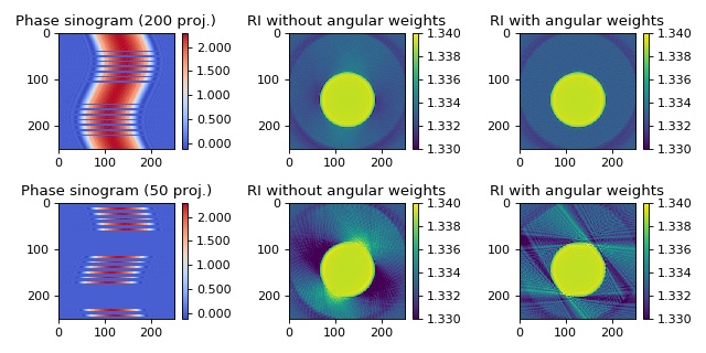
Mie cylinder with unevenly spaced angles
Angular weighting can significantly improve reconstruction quality when the angular projections are sampled at non-equidistant intervals [TPM81]. The in silico data set was created with the softare miefield. The data are 1D projections of a non-centered cylinder of constant refractive index 1.339 embedded in water with refractive index 1.333. The first column shows the used sinograms (missing angles are displayed as zeros) that were created from the original sinogram with 250 projections. The second column shows the reconstruction without angular weights and the third column shows the reconstruction with angular weights. The keyword argument weight_angles was introduced in version 0.1.1.
backprop_from_mie_2d_weights_angles.py
  1import matplotlib.pylab as plt
  2import numpy as np
  3import unwrap
  4
  5import odtbrain as odt
  6
  7from example_helper import load_data
  8
  9
 10sino, angles, cfg = load_data("mie_2d_noncentered_cylinder_A250_R2.zip",
 11                              f_angles="mie_angles.txt",
 12                              f_sino_real="sino_real.txt",
 13                              f_sino_imag="sino_imag.txt",
 14                              f_info="mie_info.txt")
 15A, size = sino.shape
 16
 17# background sinogram computed with Mie theory
 18# miefield.GetSinogramCylinderRotation(radius, nmed, nmed, lD, lC, size, A,res)
 19u0 = load_data("mie_2d_noncentered_cylinder_A250_R2.zip",
 20               f_sino_imag="u0_imag.txt",
 21               f_sino_real="u0_real.txt")
 22# create 2d array
 23u0 = np.tile(u0, size).reshape(A, size).transpose()
 24
 25# background field necessary to compute initial born field
 26# u0_single = mie.GetFieldCylinder(radius, nmed, nmed, lD, size, res)
 27u0_single = load_data("mie_2d_noncentered_cylinder_A250_R2.zip",
 28                      f_sino_imag="u0_single_imag.txt",
 29                      f_sino_real="u0_single_real.txt")
 30
 31
 32print("Example: Backpropagation from 2D FDTD simulations")
 33print("Refractive index of medium:", cfg["nmed"])
 34print("Measurement position from object center:", cfg["lD"])
 35print("Wavelength sampling:", cfg["res"])
 36print("Performing backpropagation.")
 37
 38# Set measurement parameters
 39# Compute scattered field from cylinder
 40radius = cfg["radius"]  # wavelengths
 41nmed = cfg["nmed"]
 42ncyl = cfg["ncyl"]
 43
 44lD = cfg["lD"]  # measurement distance in wavelengths
 45lC = cfg["lC"]  # displacement from center of image
 46size = cfg["size"]
 47res = cfg["res"]  # px/wavelengths
 48A = cfg["A"]  # number of projections
 49
 50x = np.arange(size) - size / 2.0
 51X, Y = np.meshgrid(x, x)
 52rad_px = radius * res
 53phantom = np.array(((Y - lC * res)**2 + X**2) < rad_px **
 54                   2, dtype=np.float) * (ncyl - nmed) + nmed
 55
 56u_sinR = odt.sinogram_as_rytov(sino / u0)
 57
 58# Rytov 200 projections
 59# remove 50 projections from total of 250 projections
 60remove200 = np.argsort(angles % .0002)[:50]
 61angles200 = np.delete(angles, remove200, axis=0)
 62u_sinR200 = np.delete(u_sinR, remove200, axis=0)
 63ph200 = unwrap.unwrap(np.angle(sino / u0))
 64ph200[remove200] = 0
 65
 66fR200 = odt.backpropagate_2d(u_sinR200, angles200, res, nmed, lD*res)
 67nR200 = odt.odt_to_ri(fR200, res, nmed)
 68fR200nw = odt.backpropagate_2d(u_sinR200, angles200, res, nmed, lD*res,
 69                               weight_angles=False)
 70nR200nw = odt.odt_to_ri(fR200nw, res, nmed)
 71
 72# Rytov 50 projections
 73remove50 = np.argsort(angles % .0002)[:200]
 74angles50 = np.delete(angles, remove50, axis=0)
 75u_sinR50 = np.delete(u_sinR, remove50, axis=0)
 76ph50 = unwrap.unwrap(np.angle(sino / u0))
 77ph50[remove50] = 0
 78
 79fR50 = odt.backpropagate_2d(u_sinR50, angles50, res, nmed, lD*res)
 80nR50 = odt.odt_to_ri(fR50, res, nmed)
 81fR50nw = odt.backpropagate_2d(u_sinR50, angles50, res, nmed, lD*res,
 82                              weight_angles=False)
 83nR50nw = odt.odt_to_ri(fR50nw, res, nmed)
 84
 85# prepare plot
 86kw_ri = {"vmin": 1.330,
 87         "vmax": 1.340}
 88
 89kw_ph = {"vmin": np.min(np.array([ph200, ph50])),
 90         "vmax": np.max(np.array([ph200, ph50])),
 91         "cmap": "coolwarm"}
 92
 93fig, axes = plt.subplots(2, 3, figsize=(8, 4))
 94axes = np.array(axes).flatten()
 95
 96phmap = axes[0].imshow(ph200, **kw_ph)
 97axes[0].set_title("Phase sinogram (200 proj.)")
 98
 99rimap = axes[1].imshow(nR200nw.real, **kw_ri)
100axes[1].set_title("RI without angular weights")
101
102axes[2].imshow(nR200.real, **kw_ri)
103axes[2].set_title("RI with angular weights")
104
105axes[3].imshow(ph50, **kw_ph)
106axes[3].set_title("Phase sinogram (50 proj.)")
107
108axes[4].imshow(nR50nw.real, **kw_ri)
109axes[4].set_title("RI without angular weights")
110
111axes[5].imshow(nR50.real, **kw_ri)
112axes[5].set_title("RI with angular weights")
113
114# color bars
115cbkwargs = {"fraction": 0.045,
116            "format": "%.3f"}
117plt.colorbar(phmap, ax=axes[0], **cbkwargs)
118plt.colorbar(phmap, ax=axes[3], **cbkwargs)
119plt.colorbar(rimap, ax=axes[1], **cbkwargs)
120plt.colorbar(rimap, ax=axes[2], **cbkwargs)
121plt.colorbar(rimap, ax=axes[5], **cbkwargs)
122plt.colorbar(rimap, ax=axes[4], **cbkwargs)
123
124plt.tight_layout()
125plt.show()
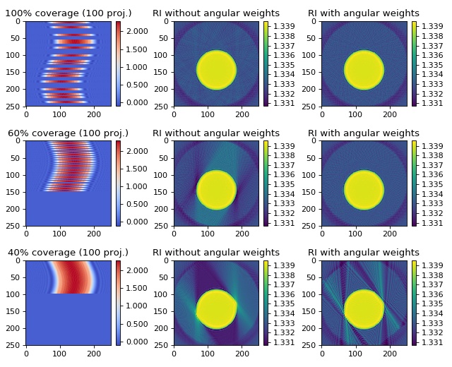
Mie cylinder with incomplete angular coverage
This example illustrates how the backpropagation algorithm of ODTbrain handles incomplete angular coverage. All examples use 100 projections at 100%, 60%, and 40% total angular coverage. The keyword argument weight_angles that invokes angular weighting is set to True by default. The in silico data set was created with the softare miefield. The data are 1D projections of a non-centered cylinder of constant refractive index 1.339 embedded in water with refractive index 1.333. The first column shows the used sinograms (missing angles are displayed as zeros) that were created from the original sinogram with 250 projections. The second column shows the reconstruction without angular weights and the third column shows the reconstruction with angular weights. The keyword argument weight_angles was introduced in version 0.1.1.
A 180 degree coverage results in a good reconstruction of the object. Angular weighting as implemented in the backpropagation algorithm of ODTbrain automatically addresses uneven and incomplete angular coverage.
backprop_from_mie_2d_incomplete_coverage.py
  1import matplotlib.pylab as plt
  2import numpy as np
  3
  4import odtbrain as odt
  5
  6from example_helper import load_data
  7
  8sino, angles, cfg = load_data("mie_2d_noncentered_cylinder_A250_R2.zip",
  9                              f_angles="mie_angles.txt",
 10                              f_sino_real="sino_real.txt",
 11                              f_sino_imag="sino_imag.txt",
 12                              f_info="mie_info.txt")
 13A, size = sino.shape
 14
 15# background sinogram computed with Mie theory
 16# miefield.GetSinogramCylinderRotation(radius, nmed, nmed, lD, lC, size, A,res)
 17u0 = load_data("mie_2d_noncentered_cylinder_A250_R2.zip",
 18               f_sino_imag="u0_imag.txt",
 19               f_sino_real="u0_real.txt")
 20# create 2d array
 21u0 = np.tile(u0, size).reshape(A, size).transpose()
 22
 23# background field necessary to compute initial born field
 24# u0_single = mie.GetFieldCylinder(radius, nmed, nmed, lD, size, res)
 25u0_single = load_data("mie_2d_noncentered_cylinder_A250_R2.zip",
 26                      f_sino_imag="u0_single_imag.txt",
 27                      f_sino_real="u0_single_real.txt")
 28
 29print("Example: Backpropagation from 2D FDTD simulations")
 30print("Refractive index of medium:", cfg["nmed"])
 31print("Measurement position from object center:", cfg["lD"])
 32print("Wavelength sampling:", cfg["res"])
 33print("Performing backpropagation.")
 34
 35# Set measurement parameters
 36# Compute scattered field from cylinder
 37radius = cfg["radius"]  # wavelengths
 38nmed = cfg["nmed"]
 39ncyl = cfg["ncyl"]
 40
 41lD = cfg["lD"]  # measurement distance in wavelengths
 42lC = cfg["lC"]  # displacement from center of image
 43size = cfg["size"]
 44res = cfg["res"]  # px/wavelengths
 45A = cfg["A"]  # number of projections
 46
 47x = np.arange(size) - size / 2.0
 48X, Y = np.meshgrid(x, x)
 49rad_px = radius * res
 50phantom = np.array(((Y - lC * res)**2 + X**2) < rad_px **
 51                   2, dtype=np.float) * (ncyl - nmed) + nmed
 52
 53u_sinR = odt.sinogram_as_rytov(sino / u0)
 54
 55# Rytov 100 projections evenly distributed
 56removeeven = np.argsort(angles % .002)[:150]
 57angleseven = np.delete(angles, removeeven, axis=0)
 58u_sinReven = np.delete(u_sinR, removeeven, axis=0)
 59pheven = odt.sinogram_as_radon(sino / u0)
 60pheven[removeeven] = 0
 61
 62fReven = odt.backpropagate_2d(u_sinReven, angleseven, res, nmed, lD * res)
 63nReven = odt.odt_to_ri(fReven, res, nmed)
 64fRevennw = odt.backpropagate_2d(
 65    u_sinReven, angleseven, res, nmed, lD * res, weight_angles=False)
 66nRevennw = odt.odt_to_ri(fRevennw, res, nmed)
 67
 68# Rytov 100 projections more than 180
 69removemiss = 249 - \
 70    np.concatenate((np.arange(100), 100 + np.arange(150)[::3]))
 71anglesmiss = np.delete(angles, removemiss, axis=0)
 72u_sinRmiss = np.delete(u_sinR, removemiss, axis=0)
 73phmiss = odt.sinogram_as_radon(sino / u0)
 74phmiss[removemiss] = 0
 75
 76fRmiss = odt.backpropagate_2d(u_sinRmiss, anglesmiss, res, nmed, lD * res)
 77nRmiss = odt.odt_to_ri(fRmiss, res, nmed)
 78fRmissnw = odt.backpropagate_2d(
 79    u_sinRmiss, anglesmiss, res, nmed, lD * res, weight_angles=False)
 80nRmissnw = odt.odt_to_ri(fRmissnw, res, nmed)
 81
 82# Rytov 100 projections less than 180
 83removebad = 249 - np.arange(150)
 84anglesbad = np.delete(angles, removebad, axis=0)
 85u_sinRbad = np.delete(u_sinR, removebad, axis=0)
 86phbad = odt.sinogram_as_radon(sino / u0)
 87phbad[removebad] = 0
 88
 89fRbad = odt.backpropagate_2d(u_sinRbad, anglesbad, res, nmed, lD * res)
 90nRbad = odt.odt_to_ri(fRbad, res, nmed)
 91fRbadnw = odt.backpropagate_2d(
 92    u_sinRbad, anglesbad, res, nmed, lD * res, weight_angles=False)
 93nRbadnw = odt.odt_to_ri(fRbadnw, res, nmed)
 94
 95# prepare plot
 96kw_ri = {"vmin": np.min(np.array([phantom, nRmiss.real, nReven.real])),
 97         "vmax": np.max(np.array([phantom, nRmiss.real, nReven.real]))}
 98
 99kw_ph = {"vmin": np.min(np.array([pheven, phmiss])),
100         "vmax": np.max(np.array([pheven, phmiss])),
101         "cmap": "coolwarm"}
102
103fig, axes = plt.subplots(3, 3, figsize=(8, 6.5))
104
105axes[0, 0].set_title("100% coverage ({} proj.)".format(angleseven.shape[0]))
106phmap = axes[0, 0].imshow(pheven, **kw_ph)
107
108axes[0, 1].set_title("RI without angular weights")
109rimap = axes[0, 1].imshow(nRevennw.real, **kw_ri)
110
111axes[0, 2].set_title("RI with angular weights")
112rimap = axes[0, 2].imshow(nReven.real, **kw_ri)
113
114axes[1, 0].set_title("60% coverage ({} proj.)".format(anglesmiss.shape[0]))
115axes[1, 0].imshow(phmiss, **kw_ph)
116
117axes[1, 1].set_title("RI without angular weights")
118axes[1, 1].imshow(nRmissnw.real, **kw_ri)
119
120axes[1, 2].set_title("RI with angular weights")
121axes[1, 2].imshow(nRmiss.real, **kw_ri)
122
123axes[2, 0].set_title("40% coverage ({} proj.)".format(anglesbad.shape[0]))
124axes[2, 0].imshow(phbad, **kw_ph)
125
126axes[2, 1].set_title("RI without angular weights")
127axes[2, 1].imshow(nRbadnw.real, **kw_ri)
128
129axes[2, 2].set_title("RI with angular weights")
130axes[2, 2].imshow(nRbad.real, **kw_ri)
131
132# color bars
133cbkwargs = {"fraction": 0.045,
134            "format": "%.3f"}
135plt.colorbar(phmap, ax=axes[0, 0], **cbkwargs)
136plt.colorbar(phmap, ax=axes[1, 0], **cbkwargs)
137plt.colorbar(phmap, ax=axes[2, 0], **cbkwargs)
138plt.colorbar(rimap, ax=axes[0, 1], **cbkwargs)
139plt.colorbar(rimap, ax=axes[1, 1], **cbkwargs)
140plt.colorbar(rimap, ax=axes[2, 1], **cbkwargs)
141plt.colorbar(rimap, ax=axes[0, 2], **cbkwargs)
142plt.colorbar(rimap, ax=axes[1, 2], **cbkwargs)
143plt.colorbar(rimap, ax=axes[2, 2], **cbkwargs)
144
145plt.tight_layout()
146plt.show()
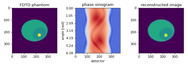
FDTD cell phantom
The in silico data set was created with the FDTD software meep. The data are 1D projections of a 2D refractive index phantom. The reconstruction of the refractive index with the Rytov approximation is in good agreement with the phantom that was used in the simulation.
 1import matplotlib.pylab as plt
 2import numpy as np
 3import odtbrain as odt
 4
 5from example_helper import load_data
 6
 7
 8sino, angles, phantom, cfg = load_data("fdtd_2d_sino_A100_R13.zip",
 9                                       f_angles="fdtd_angles.txt",
10                                       f_sino_imag="fdtd_imag.txt",
11                                       f_sino_real="fdtd_real.txt",
12                                       f_info="fdtd_info.txt",
13                                       f_phantom="fdtd_phantom.txt",
14                                       )
15
16print("Example: Backpropagation from 2D FDTD simulations")
17print("Refractive index of medium:", cfg["nm"])
18print("Measurement position from object center:", cfg["lD"])
19print("Wavelength sampling:", cfg["res"])
20print("Performing backpropagation.")
21
22# Apply the Rytov approximation
23sino_rytov = odt.sinogram_as_rytov(sino)
24
25# perform backpropagation to obtain object function f
26f = odt.backpropagate_2d(uSin=sino_rytov,
27                         angles=angles,
28                         res=cfg["res"],
29                         nm=cfg["nm"],
30                         lD=cfg["lD"] * cfg["res"]
31                         )
32
33# compute refractive index n from object function
34n = odt.odt_to_ri(f, res=cfg["res"], nm=cfg["nm"])
35
36# compare phantom and reconstruction in plot
37fig, axes = plt.subplots(1, 3, figsize=(8, 2.8))
38
39axes[0].set_title("FDTD phantom")
40axes[0].imshow(phantom, vmin=phantom.min(), vmax=phantom.max())
41sino_phase = np.unwrap(np.angle(sino), axis=1)
42
43axes[1].set_title("phase sinogram")
44axes[1].imshow(sino_phase, vmin=sino_phase.min(), vmax=sino_phase.max(),
45               aspect=sino.shape[1] / sino.shape[0],
46               cmap="coolwarm")
47axes[1].set_xlabel("detector")
48axes[1].set_ylabel("angle [rad]")
49
50axes[2].set_title("reconstructed image")
51axes[2].imshow(n.real, vmin=phantom.min(), vmax=phantom.max())
52
53# set y ticks for sinogram
54labels = np.linspace(0, 2 * np.pi, len(axes[1].get_yticks()))
55labels = ["{:.2f}".format(i) for i in labels]
56axes[1].set_yticks(np.linspace(0, len(angles), len(labels)))
57axes[1].set_yticklabels(labels)
58
59plt.tight_layout()
60plt.show()