3D examples
These examples require raw data which are automatically
downloaded from the source repository by the script
example_helper.py.
Please make sure that this script is present in the example
script folder.
Note
The if __name__ == "__main__" guard is necessary on Windows and macOS
which spawn new processes instead of forking the current process.
The 3D backpropagation algorithm makes use of multiprocessing.Pool.
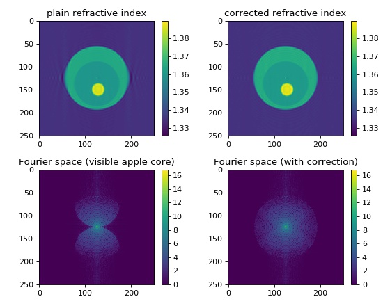
Missing apple core correction
The missing apple core [VDYH09] is a phenomenon in diffraction tomography that is a result of the fact the the Fourier space is not filled completely when the sample is rotated only about a single axis. The resulting artifacts include ringing and blurring in the reconstruction parallel to the original rotation axis. By enforcing constraints (refractive index real-valued and larger than the surrounding medium), these artifacts can be attenuated.
This example generates an artificial sinogram using the Python library cellsino (The example parameters are reused from this example). The sinogram is then reconstructed with the backpropagation algorithm and the missing apple core correction is applied.
Note
The missing apple core correction odtbrain.apple.correct()
was implemented in version 0.3.0 and is thus not used in the
older examples.
backprop_from_rytov_3d_phantom_apple.py
 1import matplotlib.pylab as plt
 2import numpy as np
 3
 4import cellsino
 5import odtbrain as odt
 6
 7
 8if __name__ == "__main__":
 9    # number of sinogram angles
10    num_ang = 160
11    # sinogram acquisition angles
12    angles = np.linspace(0, 2*np.pi, num_ang, endpoint=False)
13    # detector grid size
14    grid_size = (250, 250)
15    # vacuum wavelength [m]
16    wavelength = 550e-9
17    # pixel size [m]
18    pixel_size = 0.08e-6
19    # refractive index of the surrounding medium
20    medium_index = 1.335
21
22    # initialize cell phantom
23    phantom = cellsino.phantoms.SimpleCell()
24
25    # initialize sinogram with geometric parameters
26    sino = cellsino.Sinogram(phantom=phantom,
27                             wavelength=wavelength,
28                             pixel_size=pixel_size,
29                             grid_size=grid_size)
30
31    # compute sinogram (field with Rytov approximation and fluorescence)
32    sino = sino.compute(angles=angles, propagator="rytov", mode="field")
33
34    # reconstruction of refractive index
35    sino_rytov = odt.sinogram_as_rytov(sino)
36    f = odt.backpropagate_3d(uSin=sino_rytov,
37                             angles=angles,
38                             res=wavelength/pixel_size,
39                             nm=medium_index)
40
41    ri = odt.odt_to_ri(f=f,
42                       res=wavelength/pixel_size,
43                       nm=medium_index)
44
45    # apple core correction
46    fc = odt.apple.correct(f=f,
47                           res=wavelength/pixel_size,
48                           nm=medium_index,
49                           method="sh")
50
51    ric = odt.odt_to_ri(f=fc,
52                        res=wavelength/pixel_size,
53                        nm=medium_index)
54
55    # plotting
56    idx = ri.shape[2] // 2
57
58    # log-scaled power spectra
59    ft = np.log(1 + np.abs(np.fft.fftshift(np.fft.fftn(ri))))
60    ftc = np.log(1 + np.abs(np.fft.fftshift(np.fft.fftn(ric))))
61
62    plt.figure(figsize=(7, 5.5))
63
64    plotkwri = {"vmax": ri.real.max(),
65                "vmin": ri.real.min(),
66                "interpolation": "none",
67                }
68
69    plotkwft = {"vmax": ft.max(),
70                "vmin": 0,
71                "interpolation": "none",
72                }
73
74    ax1 = plt.subplot(221, title="plain refractive index")
75    mapper = ax1.imshow(ri[:, :, idx].real, **plotkwri)
76    plt.colorbar(mappable=mapper, ax=ax1)
77
78    ax2 = plt.subplot(222, title="corrected refractive index")
79    mapper = ax2.imshow(ric[:, :, idx].real, **plotkwri)
80    plt.colorbar(mappable=mapper, ax=ax2)
81
82    ax3 = plt.subplot(223, title="Fourier space (visible apple core)")
83    mapper = ax3.imshow(ft[:, :, idx], **plotkwft)
84    plt.colorbar(mappable=mapper, ax=ax3)
85
86    ax4 = plt.subplot(224, title="Fourier space (with correction)")
87    mapper = ax4.imshow(ftc[:, :, idx], **plotkwft)
88    plt.colorbar(mappable=mapper, ax=ax4)
89
90    plt.tight_layout()
91    plt.show()
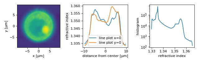
HL60 cell
The quantitative phase data of an HL60 S/4 cell were recorded using QLSI. The original dataset was used in a previous publication [SCG+17] to illustrate the capabilities of combined fluorescence and refractive index tomography.
The example data set is already aligned and background-corrected as described in the original publication and the fluorescence data are not included. The lzma-archive contains the sinogram data stored in the qpimage file format and the rotational positions of each sinogram image as a text file.
The figure reproduces parts of figure 4 of the original manuscript. Note that minor deviations from the original figure can be attributed to the strong compression (scale offset filter) and due to the fact that the original sinogram images were cropped from 196x196 px to 140x140 px (which in particular affects the background-part of the refractive index histogram).
The raw data is available on figshare <https://doi.org/10.6084/m9.figshare.8055407.v1> (hl60_sinogram_qpi.h5).
 1import pathlib
 2import tarfile
 3import tempfile
 4
 5import matplotlib.pylab as plt
 6import numpy as np
 7import odtbrain as odt
 8import qpimage
 9
10from example_helper import get_file, extract_lzma
11
12
13if __name__ == "__main__":
14    # ascertain the data
15    path = get_file("qlsi_3d_hl60-cell_A140.tar.lzma")
16    tarf = extract_lzma(path)
17    tdir = tempfile.mkdtemp(prefix="odtbrain_example_")
18
19    with tarfile.open(tarf) as tf:
20        tf.extract("series.h5", path=tdir)
21        angles = np.loadtxt(tf.extractfile("angles.txt"))
22
23    # extract the complex field sinogram from the qpimage series data
24    h5file = pathlib.Path(tdir) / "series.h5"
25    with qpimage.QPSeries(h5file=h5file, h5mode="r") as qps:
26        qp0 = qps[0]
27        meta = qp0.meta
28        sino = np.zeros((len(qps), qp0.shape[0], qp0.shape[1]),
29                        dtype=np.complex)
30        for ii in range(len(qps)):
31            sino[ii] = qps[ii].field
32
33    # perform backgpropagation
34    u_sinR = odt.sinogram_as_rytov(sino)
35    res = meta["wavelength"] / meta["pixel size"]
36    nm = meta["medium index"]
37
38    fR = odt.backpropagate_3d(uSin=u_sinR,
39                              angles=angles,
40                              res=res,
41                              nm=nm)
42
43    ri = odt.odt_to_ri(fR, res, nm)
44
45    # plot results
46    ext = meta["pixel size"] * 1e6 * 70
47    kw = {"vmin": ri.real.min(),
48          "vmax": ri.real.max(),
49          "extent": [-ext, ext, -ext, ext]}
50    fig, axes = plt.subplots(1, 3, figsize=(8, 2.5))
51    axes[0].imshow(ri[70, :, :].real, **kw)
52    axes[0].set_xlabel("x [µm]")
53    axes[0].set_ylabel("y [µm]")
54
55    x = np.linspace(-ext, ext, 140)
56    axes[1].plot(x, ri[70, :, 70], label="line plot x=0")
57    axes[1].plot(x, ri[70, 70, :], label="line plot y=0")
58    axes[1].set_xlabel("distance from center [µm]")
59    axes[1].set_ylabel("refractive index")
60    axes[1].legend()
61
62    hist, xh = np.histogram(ri.real, bins=100)
63    axes[2].plot(xh[1:], hist)
64    axes[2].set_yscale('log')
65    axes[2].set_xlabel("refractive index")
66    axes[2].set_ylabel("histogram")
67
68    plt.tight_layout()
69    plt.show()
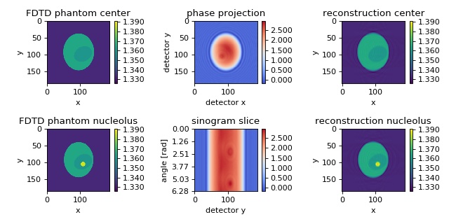
FDTD cell phantom
The in silico data set was created with the FDTD software meep. The data are 2D projections of a 3D refractive index phantom. The reconstruction of the refractive index with the Rytov approximation is in good agreement with the phantom that was used in the simulation. The data are downsampled by a factor of two. The rotational axis is the y-axis. A total of 180 projections are used for the reconstruction. A detailed description of this phantom is given in [MSG15a].
 1import matplotlib.pylab as plt
 2import numpy as np
 3
 4import odtbrain as odt
 5
 6from example_helper import load_data
 7
 8
 9if __name__ == "__main__":
10    sino, angles, phantom, cfg = \
11        load_data("fdtd_3d_sino_A180_R6.500.tar.lzma")
12
13    A = angles.shape[0]
14
15    print("Example: Backpropagation from 3D FDTD simulations")
16    print("Refractive index of medium:", cfg["nm"])
17    print("Measurement position from object center:", cfg["lD"])
18    print("Wavelength sampling:", cfg["res"])
19    print("Number of projections:", A)
20    print("Performing backpropagation.")
21
22    # Apply the Rytov approximation
23    sinoRytov = odt.sinogram_as_rytov(sino)
24
25    # perform backpropagation to obtain object function f
26    f = odt.backpropagate_3d(uSin=sinoRytov,
27                             angles=angles,
28                             res=cfg["res"],
29                             nm=cfg["nm"],
30                             lD=cfg["lD"]
31                             )
32
33    # compute refractive index n from object function
34    n = odt.odt_to_ri(f, res=cfg["res"], nm=cfg["nm"])
35
36    sx, sy, sz = n.shape
37    px, py, pz = phantom.shape
38
39    sino_phase = np.angle(sino)
40
41    # compare phantom and reconstruction in plot
42    fig, axes = plt.subplots(2, 3, figsize=(8, 4))
43    kwri = {"vmin": n.real.min(), "vmax": n.real.max()}
44    kwph = {"vmin": sino_phase.min(), "vmax": sino_phase.max(),
45            "cmap": "coolwarm"}
46
47    # Phantom
48    axes[0, 0].set_title("FDTD phantom center")
49    rimap = axes[0, 0].imshow(phantom[px // 2], **kwri)
50    axes[0, 0].set_xlabel("x")
51    axes[0, 0].set_ylabel("y")
52
53    axes[1, 0].set_title("FDTD phantom nucleolus")
54    axes[1, 0].imshow(phantom[int(px / 2 + 2 * cfg["res"])], **kwri)
55    axes[1, 0].set_xlabel("x")
56    axes[1, 0].set_ylabel("y")
57
58    # Sinogram
59    axes[0, 1].set_title("phase projection")
60    phmap = axes[0, 1].imshow(sino_phase[A // 2, :, :], **kwph)
61    axes[0, 1].set_xlabel("detector x")
62    axes[0, 1].set_ylabel("detector y")
63
64    axes[1, 1].set_title("sinogram slice")
65    axes[1, 1].imshow(sino_phase[:, :, sino.shape[2] // 2],
66                      aspect=sino.shape[1] / sino.shape[0], **kwph)
67    axes[1, 1].set_xlabel("detector y")
68    axes[1, 1].set_ylabel("angle [rad]")
69    # set y ticks for sinogram
70    labels = np.linspace(0, 2 * np.pi, len(axes[1, 1].get_yticks()))
71    labels = ["{:.2f}".format(i) for i in labels]
72    axes[1, 1].set_yticks(np.linspace(0, len(angles), len(labels)))
73    axes[1, 1].set_yticklabels(labels)
74
75    axes[0, 2].set_title("reconstruction center")
76    axes[0, 2].imshow(n[sx // 2].real, **kwri)
77    axes[0, 2].set_xlabel("x")
78    axes[0, 2].set_ylabel("y")
79
80    axes[1, 2].set_title("reconstruction nucleolus")
81    axes[1, 2].imshow(n[int(sx / 2 + 2 * cfg["res"])].real, **kwri)
82    axes[1, 2].set_xlabel("x")
83    axes[1, 2].set_ylabel("y")
84
85    # color bars
86    cbkwargs = {"fraction": 0.045,
87                "format": "%.3f"}
88    plt.colorbar(phmap, ax=axes[0, 1], **cbkwargs)
89    plt.colorbar(phmap, ax=axes[1, 1], **cbkwargs)
90    plt.colorbar(rimap, ax=axes[0, 0], **cbkwargs)
91    plt.colorbar(rimap, ax=axes[1, 0], **cbkwargs)
92    plt.colorbar(rimap, ax=axes[0, 2], **cbkwargs)
93    plt.colorbar(rimap, ax=axes[1, 2], **cbkwargs)
94
95    plt.tight_layout()
96    plt.show()
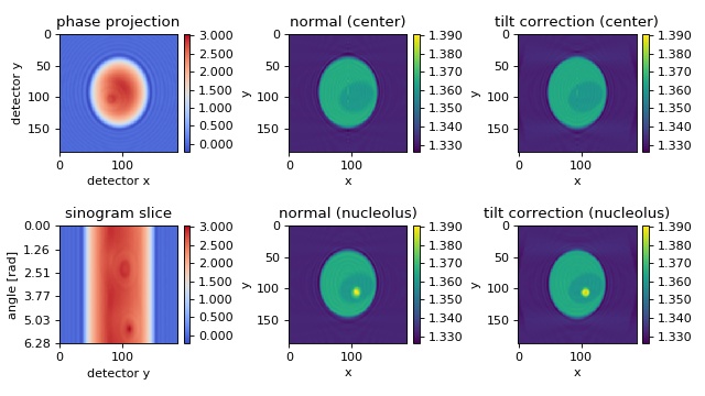
FDTD cell phantom with tilted axis of rotation
The in silico data set was created with the
FDTD software meep. The data
are 2D projections of a 3D refractive index phantom that is rotated
about an axis which is tilted by 0.2 rad (11.5 degrees) with respect
to the imaging plane. The example showcases the method
odtbrain.backpropagate_3d_tilted() which takes into account
such a tilted axis of rotation. The data are downsampled by a factor
of two. A total of 220 projections are used for the reconstruction.
Note that the information required for reconstruction decreases as the
tilt angle increases. If the tilt angle is 90 degrees w.r.t. the
imaging plane, then we get a rotating image of a cell (not images of a
rotating cell) and tomographic reconstruction is impossible. A brief
description of this algorithm is given in [MSCG15].
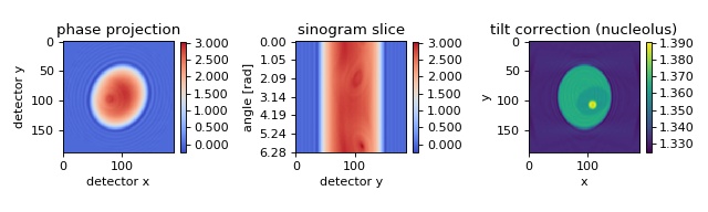
The first column shows the measured phase, visualizing the tilt (compare to other examples). The second column shows a reconstruction that does not take into account the tilted axis of rotation; the result is a blurry reconstruction. The third column shows the improved reconstruction; the known tilted axis of rotation is used in the reconstruction process.
backprop_from_fdtd_3d_tilted.py
  1import matplotlib.pylab as plt
  2import numpy as np
  3
  4import odtbrain as odt
  5
  6from example_helper import load_data
  7
  8
  9if __name__ == "__main__":
 10    sino, angles, phantom, cfg = \
 11        load_data("fdtd_3d_sino_A220_R6.500_tiltyz0.2.tar.lzma")
 12
 13    A = angles.shape[0]
 14
 15    print("Example: Backpropagation from 3D FDTD simulations")
 16    print("Refractive index of medium:", cfg["nm"])
 17    print("Measurement position from object center:", cfg["lD"])
 18    print("Wavelength sampling:", cfg["res"])
 19    print("Axis tilt in y-z direction:", cfg["tilt_yz"])
 20    print("Number of projections:", A)
 21
 22    print("Performing normal backpropagation.")
 23    # Apply the Rytov approximation
 24    sinoRytov = odt.sinogram_as_rytov(sino)
 25
 26    # Perform naive backpropagation
 27    f_naiv = odt.backpropagate_3d(uSin=sinoRytov,
 28                                  angles=angles,
 29                                  res=cfg["res"],
 30                                  nm=cfg["nm"],
 31                                  lD=cfg["lD"]
 32                                  )
 33
 34    print("Performing tilted backpropagation.")
 35    # Determine tilted axis
 36    tilted_axis = [0, np.cos(cfg["tilt_yz"]), np.sin(cfg["tilt_yz"])]
 37
 38    # Perform tilted backpropagation
 39    f_tilt = odt.backpropagate_3d_tilted(uSin=sinoRytov,
 40                                         angles=angles,
 41                                         res=cfg["res"],
 42                                         nm=cfg["nm"],
 43                                         lD=cfg["lD"],
 44                                         tilted_axis=tilted_axis,
 45                                         )
 46
 47    # compute refractive index n from object function
 48    n_naiv = odt.odt_to_ri(f_naiv, res=cfg["res"], nm=cfg["nm"])
 49    n_tilt = odt.odt_to_ri(f_tilt, res=cfg["res"], nm=cfg["nm"])
 50
 51    sx, sy, sz = n_tilt.shape
 52    px, py, pz = phantom.shape
 53
 54    sino_phase = np.angle(sino)
 55
 56    # compare phantom and reconstruction in plot
 57    fig, axes = plt.subplots(2, 3, figsize=(8, 4.5))
 58    kwri = {"vmin": n_tilt.real.min(), "vmax": n_tilt.real.max()}
 59    kwph = {"vmin": sino_phase.min(), "vmax": sino_phase.max(),
 60            "cmap": "coolwarm"}
 61
 62    # Sinogram
 63    axes[0, 0].set_title("phase projection")
 64    phmap = axes[0, 0].imshow(sino_phase[A // 2, :, :], **kwph)
 65    axes[0, 0].set_xlabel("detector x")
 66    axes[0, 0].set_ylabel("detector y")
 67
 68    axes[1, 0].set_title("sinogram slice")
 69    axes[1, 0].imshow(sino_phase[:, :, sino.shape[2] // 2],
 70                      aspect=sino.shape[1] / sino.shape[0], **kwph)
 71    axes[1, 0].set_xlabel("detector y")
 72    axes[1, 0].set_ylabel("angle [rad]")
 73    # set y ticks for sinogram
 74    labels = np.linspace(0, 2 * np.pi, len(axes[1, 1].get_yticks()))
 75    labels = ["{:.2f}".format(i) for i in labels]
 76    axes[1, 0].set_yticks(np.linspace(0, len(angles), len(labels)))
 77    axes[1, 0].set_yticklabels(labels)
 78
 79    axes[0, 1].set_title("normal (center)")
 80    rimap = axes[0, 1].imshow(n_naiv[sx // 2].real, **kwri)
 81    axes[0, 1].set_xlabel("x")
 82    axes[0, 1].set_ylabel("y")
 83
 84    axes[1, 1].set_title("normal (nucleolus)")
 85    axes[1, 1].imshow(n_naiv[int(sx / 2 + 2 * cfg["res"])].real, **kwri)
 86    axes[1, 1].set_xlabel("x")
 87    axes[1, 1].set_ylabel("y")
 88
 89    axes[0, 2].set_title("tilt correction (center)")
 90    axes[0, 2].imshow(n_tilt[sx // 2].real, **kwri)
 91    axes[0, 2].set_xlabel("x")
 92    axes[0, 2].set_ylabel("y")
 93
 94    axes[1, 2].set_title("tilt correction (nucleolus)")
 95    axes[1, 2].imshow(n_tilt[int(sx / 2 + 2 * cfg["res"])].real, **kwri)
 96    axes[1, 2].set_xlabel("x")
 97    axes[1, 2].set_ylabel("y")
 98
 99    # color bars
100    cbkwargs = {"fraction": 0.045,
101                "format": "%.3f"}
102    plt.colorbar(phmap, ax=axes[0, 0], **cbkwargs)
103    plt.colorbar(phmap, ax=axes[1, 0], **cbkwargs)
104    plt.colorbar(rimap, ax=axes[0, 1], **cbkwargs)
105    plt.colorbar(rimap, ax=axes[1, 1], **cbkwargs)
106    plt.colorbar(rimap, ax=axes[0, 2], **cbkwargs)
107    plt.colorbar(rimap, ax=axes[1, 2], **cbkwargs)
108
109    plt.tight_layout()
110    plt.show()
FDTD cell phantom with tilted and rolled axis of rotation
The in silico data set was created with the FDTD software meep. The data are 2D projections of a 3D refractive index phantom that is rotated about an axis which is tilted by 0.2 rad (11.5 degrees) with respect to the imaging plane and rolled by -.42 rad (-24.1 degrees) within the imaging plane. The data are the same as were used in the previous example. A brief description of this algorithm is given in [MSCG15].
backprop_from_fdtd_3d_tilted2.py
  1import matplotlib.pylab as plt
  2import numpy as np
  3from scipy.ndimage import rotate
  4
  5import odtbrain as odt
  6
  7from example_helper import load_data
  8
  9
 10if __name__ == "__main__":
 11    sino, angles, phantom, cfg = \
 12        load_data("fdtd_3d_sino_A220_R6.500_tiltyz0.2.tar.lzma")
 13
 14    # Perform titlt by -.42 rad in detector plane
 15    rotang = -0.42
 16    rotkwargs = {"mode": "constant",
 17                 "order": 2,
 18                 "reshape": False,
 19                 }
 20    for ii in range(len(sino)):
 21        sino[ii].real = rotate(
 22            sino[ii].real, np.rad2deg(rotang), cval=1, **rotkwargs)
 23        sino[ii].imag = rotate(
 24            sino[ii].imag, np.rad2deg(rotang), cval=0, **rotkwargs)
 25
 26    A = angles.shape[0]
 27
 28    print("Example: Backpropagation from 3D FDTD simulations")
 29    print("Refractive index of medium:", cfg["nm"])
 30    print("Measurement position from object center:", cfg["lD"])
 31    print("Wavelength sampling:", cfg["res"])
 32    print("Axis tilt in y-z direction:", cfg["tilt_yz"])
 33    print("Number of projections:", A)
 34
 35    # Apply the Rytov approximation
 36    sinoRytov = odt.sinogram_as_rytov(sino)
 37
 38    # Determine tilted axis
 39    tilted_axis = [0, np.cos(cfg["tilt_yz"]), np.sin(cfg["tilt_yz"])]
 40    rotmat = np.array([
 41        [np.cos(rotang), -np.sin(rotang), 0],
 42        [np.sin(rotang), np.cos(rotang), 0],
 43        [0, 0, 1],
 44    ])
 45    tilted_axis = np.dot(rotmat, tilted_axis)
 46
 47    print("Performing tilted backpropagation.")
 48    # Perform tilted backpropagation
 49    f_tilt = odt.backpropagate_3d_tilted(uSin=sinoRytov,
 50                                         angles=angles,
 51                                         res=cfg["res"],
 52                                         nm=cfg["nm"],
 53                                         lD=cfg["lD"],
 54                                         tilted_axis=tilted_axis,
 55                                         )
 56
 57    # compute refractive index n from object function
 58    n_tilt = odt.odt_to_ri(f_tilt, res=cfg["res"], nm=cfg["nm"])
 59
 60    sx, sy, sz = n_tilt.shape
 61    px, py, pz = phantom.shape
 62
 63    sino_phase = np.angle(sino)
 64
 65    # compare phantom and reconstruction in plot
 66    fig, axes = plt.subplots(1, 3, figsize=(8, 2.4))
 67    kwri = {"vmin": n_tilt.real.min(), "vmax": n_tilt.real.max()}
 68    kwph = {"vmin": sino_phase.min(), "vmax": sino_phase.max(),
 69            "cmap": "coolwarm"}
 70
 71    # Sinogram
 72    axes[0].set_title("phase projection")
 73    phmap = axes[0].imshow(sino_phase[A // 2, :, :], **kwph)
 74    axes[0].set_xlabel("detector x")
 75    axes[0].set_ylabel("detector y")
 76
 77    axes[1].set_title("sinogram slice")
 78    axes[1].imshow(sino_phase[:, :, sino.shape[2] // 2],
 79                   aspect=sino.shape[1] / sino.shape[0], **kwph)
 80    axes[1].set_xlabel("detector y")
 81    axes[1].set_ylabel("angle [rad]")
 82    # set y ticks for sinogram
 83    labels = np.linspace(0, 2 * np.pi, len(axes[1].get_yticks()))
 84    labels = ["{:.2f}".format(i) for i in labels]
 85    axes[1].set_yticks(np.linspace(0, len(angles), len(labels)))
 86    axes[1].set_yticklabels(labels)
 87
 88    axes[2].set_title("tilt correction (nucleolus)")
 89    rimap = axes[2].imshow(n_tilt[int(sx / 2 + 2 * cfg["res"])].real, **kwri)
 90    axes[2].set_xlabel("x")
 91    axes[2].set_ylabel("y")
 92
 93    # color bars
 94    cbkwargs = {"fraction": 0.045,
 95                "format": "%.3f"}
 96    plt.colorbar(phmap, ax=axes[0], **cbkwargs)
 97    plt.colorbar(phmap, ax=axes[1], **cbkwargs)
 98    plt.colorbar(rimap, ax=axes[2], **cbkwargs)
 99
100    plt.tight_layout()
101    plt.show()
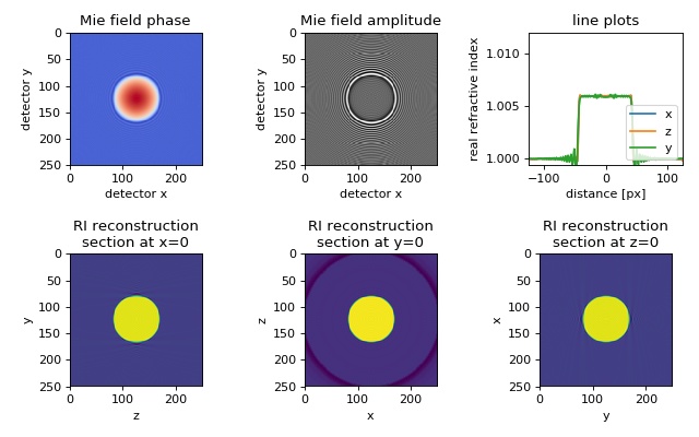
Mie sphere
The in silico data set was created with the Mie calculation software GMM-field. The data consist of a two-dimensional projection of a sphere with radius \(R=14\lambda\), refractive index \(n_\mathrm{sph}=1.006\), embedded in a medium of refractive index \(n_\mathrm{med}=1.0\) onto a detector which is \(l_\mathrm{D} = 20\lambda\) away from the center of the sphere.
The package nrefocus must be used to numerically focus
the detected field prior to the 3D backpropagation with ODTbrain.
In odtbrain.backpropagate_3d(), the parameter lD must
be set to zero (\(l_\mathrm{D}=0\)).
The figure shows the 3D reconstruction from Mie simulations of a perfect sphere using 200 projections. Missing angle artifacts are visible along the \(y\)-axis due to the \(2\pi\)-only coverage in 3D Fourier space.
backprop_from_mie_3d_sphere.py
 1import matplotlib.pylab as plt
 2import nrefocus
 3import numpy as np
 4
 5import odtbrain as odt
 6
 7from example_helper import load_data
 8
 9
10if __name__ == "__main__":
11    Ex, cfg = load_data("mie_3d_sphere_field.zip",
12                        f_sino_imag="mie_sphere_imag.txt",
13                        f_sino_real="mie_sphere_real.txt",
14                        f_info="mie_info.txt")
15
16    # Manually set number of angles:
17    A = 200
18
19    print("Example: Backpropagation from 3D Mie scattering")
20    print("Refractive index of medium:", cfg["nm"])
21    print("Measurement position from object center:", cfg["lD"])
22    print("Wavelength sampling:", cfg["res"])
23    print("Number of angles for reconstruction:", A)
24    print("Performing backpropagation.")
25
26    # Reconstruction angles
27    angles = np.linspace(0, 2 * np.pi, A, endpoint=False)
28
29    # Perform focusing
30    Ex = nrefocus.refocus(Ex,
31                          d=-cfg["lD"]*cfg["res"],
32                          nm=cfg["nm"],
33                          res=cfg["res"],
34                          )
35
36    # Create sinogram
37    u_sin = np.tile(Ex.flat, A).reshape(A, int(cfg["size"]), int(cfg["size"]))
38
39    # Apply the Rytov approximation
40    u_sinR = odt.sinogram_as_rytov(u_sin)
41
42    # Backpropagation
43    fR = odt.backpropagate_3d(uSin=u_sinR,
44                              angles=angles,
45                              res=cfg["res"],
46                              nm=cfg["nm"],
47                              lD=0,
48                              padfac=2.1,
49                              save_memory=True)
50
51    # RI computation
52    nR = odt.odt_to_ri(fR, cfg["res"], cfg["nm"])
53
54    # Plotting
55    fig, axes = plt.subplots(2, 3, figsize=(8, 5))
56    axes = np.array(axes).flatten()
57    # field
58    axes[0].set_title("Mie field phase")
59    axes[0].set_xlabel("detector x")
60    axes[0].set_ylabel("detector y")
61    axes[0].imshow(np.angle(Ex), cmap="coolwarm")
62    axes[1].set_title("Mie field amplitude")
63    axes[1].set_xlabel("detector x")
64    axes[1].set_ylabel("detector y")
65    axes[1].imshow(np.abs(Ex), cmap="gray")
66
67    # line plot
68    axes[2].set_title("line plots")
69    axes[2].set_xlabel("distance [px]")
70    axes[2].set_ylabel("real refractive index")
71    center = int(cfg["size"] / 2)
72    x = np.arange(cfg["size"]) - center
73    axes[2].plot(x, nR[:, center, center].real, label="x")
74    axes[2].plot(x, nR[center, center, :].real, label="z")
75    axes[2].plot(x, nR[center, :, center].real, label="y")
76    axes[2].legend(loc=4)
77    axes[2].set_xlim((-center, center))
78    dn = abs(cfg["nsph"] - cfg["nm"])
79    axes[2].set_ylim((cfg["nm"] - dn / 10, cfg["nsph"] + dn))
80    axes[2].ticklabel_format(useOffset=False)
81
82    # cross sections
83    axes[3].set_title("RI reconstruction\nsection at x=0")
84    axes[3].set_xlabel("z")
85    axes[3].set_ylabel("y")
86    axes[3].imshow(nR[center, :, :].real)
87
88    axes[4].set_title("RI reconstruction\nsection at y=0")
89    axes[4].set_xlabel("x")
90    axes[4].set_ylabel("z")
91    axes[4].imshow(nR[:, center, :].real)
92
93    axes[5].set_title("RI reconstruction\nsection at z=0")
94    axes[5].set_xlabel("y")
95    axes[5].set_ylabel("x")
96    axes[5].imshow(nR[:, :, center].real)
97
98    plt.tight_layout()
99    plt.show()